Conduction in the Cylindrical Geometry.pdf

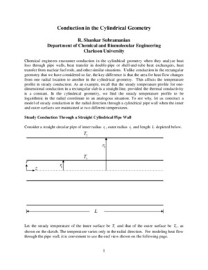
  1 Conduction in the Cylindrical Geometry R Shankar Subramanian Department of Chemical and Biomolecular Engineering Clarkson University Chemical engineers encounter conduction in the cylindrical geometry when they analyze heat loss through pipe walls, heat transfer in double-pipe or shell-and-tube heat exchangers, heat transfer from nuclear fuel rods, and other similar situations Unlike conduction in the rectangular geometry that we have considered so far, the key difference is that the area for heat flow changes from one radial location to another in the cylindrical geometry This affects the temperature  profile in steady conduction As an example, recall that the steady temperature profile for one-dimensional conduction in a rectangular slab is a straight line, provided the thermal conductivity is a constant In the cylindrical geometry, we find the steady temperature profile to be logarithmic in the radial coordinate in an analogous situation To see why, let us construct a model of steady conduction in the radial direction through a cylindrical pipe wall when the inner and outer surfaces are maintained at two different temperatures Steady Conduction Through a Straight Cylindrical Pipe Wall Consider a straight circular pipe of inner radius 1 r  , outer radius 2 r   and length  L  depicted below Let the steady temperature of the inner surface be 1 T   and that of the outer surface be 2 T  , as shown on the sketch The temperature varies only in the radial direction For modeling heat flow through the pipe wall, it is convenient to use the end view shown on the following page  z r  1 r  2 r  2 T  1 T  L  2 We use a shell balance approach Consider a cylindrical shell of inner radius r   and outer radius r r  + ∆  located within the pipe wall as shown in the sketch The shell extends the entire length  L  of the pipe Let ( ) Q r   be the radial heat flow rate at the radial location r   within the pipe wall Then, in the end view shown above, the heat flow rate into the cylindrical shell is ( ) Q r  , while the heat flow rate out of the cylindrical shell is ( ) Q r r  +∆ At steady state, ( ) ( ) Q r Q r r  = +∆ Rearrange this result after division by r  ∆  as shown below ( ) ( ) 0 Q r r Q r r  +∆ −=∆   Now take the limit as 0 r  ∆ → This leads to the simple differential equation 0 dQdr  =  Integration is straightforward, and leads to the result constant Q  =  independent of radial location The heat flow rate r  Q q A = , where  A  is the area of the cylindrical surface normal to the r   − direction, and r  q  is the heat flux in the radial direction The area of the cylindrical surface is 2  A rL π   = , where  L  is the length of the pipe From Fourier’s law, r  dT q k dr  = − Therefore, we find that 1 r  2 r  1 T  2 T r r  ∆ ( ) Q r  ( ) Q r r  +∆  3 constant dT  Ak dr  − =  Substituting for the area  A , we can write 2 constant dT rLk dr  π   − = Because 2  Lk  π    is constant, this leads to a simple differential equation for the temperature distribution in the pipe wall 1 dT r C dr  =  Here, 1 C   is a constant that needs to be determined later Rearrange this equation as 1 dr dT C r  =  and integrate both sides to yield 1 2 ln T C r C  = +  where 2 C   is another constant that needs to be determined Thus, we find that the steady state temperature distribution in the pipe wall for constant thermal conductivity is logarithmic, in contrast to conduction through a rectangular slab in which case, the steady temperature distribution was found to be linear To find the two constants in the solution, we must use boundary conditions on the temperature distribution The temperature is specified at both the inner and outer pipe wall surfaces Thus, we can write the boundary conditions as follows ( ) 1 1 T r T  =   ( ) 2 2 T r T  =  By substituting these two boundary conditions in the solution for the temperature field in turn, we obtain two equations for the undetermined constants 1 C   and 2 C  1 1 1 2 ln T C r C  = +   2 1 2 2 ln T C r C  = +  These two linear equations can be solved for the values of the constants 1 C   and 2 C   in a straightforward manner We find ( ) 1 211 2 ln / T T C r r  −=   ( ) 1 22 1 11 2 lnln / T T C T r r r  −= −  Substituting the results for the two constants in the solution for the temperature profile, followed  by rearrangement, yields the following result for the temperature distribution in the pipe wall ( )( ) 111 2 2 1 ln /ln / r r T T T T r r  −=−